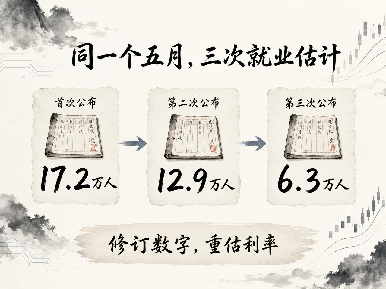
During the first half of this year, above-forecast US payroll growth repeatedly suggested a resilient labor market, only for revisions to weaken that strength. May's increase was cut successively from an initial 172,000 to 63,000.
On September 4, August again delivered a strong 162,000 gain and revised June–July additions up by a combined 55,000. From strong initial estimates to later cuts, then renewed strength and upward revisions, markets repeatedly adjusted employment and rate views.
Economic change and statistical correction became intertwined, making it harder to distinguish a genuine turn in employment from changes in the numbers previously used to judge it.
This is especially perplexing when payroll is electronic and bank transactions settle instantly. Businesses already leave extensive digital records, yet national statistics still need samples and assumptions to fill gaps. Closing the distance requires both better measurement and institutional change in data integration.
1. Repeated payroll revisions complicate rate pricing
Nonfarm payroll growth mainly measures the net monthly increase in paid jobs at nonagricultural businesses and government agencies. If 1 million jobs are added and 900,000 lost, growth is 100,000, not the number of all new hires.
The first published number is preliminary. Incomplete information normally leads to one revision in each of the following two months, incorporating late reports, corrected records and statistical-processing changes. Higher numbers are upward revisions and lower ones downward revisions.
After both regular revisions to each of the first six months of 2026, three were higher and three lower than initial estimates. Ignoring direction, the average revision was about 50,000. For months originally growing only tens of thousands, that can reverse the strength assessment.
| Month | First release | Second release | Third release |
|---|---|---|---|
| January | 13.0 | 12.6 | 16.0 |
| February | -9.2 | -13.3 | -15.6 |
| March | 17.8 | 18.5 | 21.4 |
| April | 11.5 | 17.9 | 14.8 |
| May | 17.2 | 12.9 | 6.3 |
| June | 5.7 | 2.0 | 3.1 |
Table unit: 10,000 people; negative figures indicate job losses. Numbers remove estimated regular seasonal effects. The third release completes two monthly revisions but can still change later.
May illustrates the gap: 172,000 fell to 63,000, a cumulative 109,000 reduction, about 63% of the initial estimate. April rose from 115,000 to 179,000 before falling to 148,000. The same month's employment gave signals of different strength at successive releases.
August brought markets back to a strong-jobs narrative: 162,000 versus an expected 56,000, with June–July revised up 55,000. July even changed from a 23,000 loss to a 21,000 gain.
Yet the latest June–August average was only about 71,000 monthly. Food services/drinking places and local-government education contributed roughly 62% of August's gain. One rebound cannot establish sustained faster hiring across most industries.
The effects extend beyond tables. The Fed influences borrowing costs through rates and has responsibilities for stable prices and maximum employment. Strong jobs generally reduce concern that hikes will damage employment; persistent weakness can increase the need for cuts.
Investors trade Treasuries and rate futures accordingly. Futures contracts on future interest rates can be converted into implied hike or cut probabilities. These change with news and are not policy commitments.
On February 11, January's 130,000 gain exceeded the Reuters poll's 70,000. After the report, futures-implied odds of no June rate change rose from about 25% to nearly 40%. On March 6, February unexpectedly lost 92,000 against a forecast 59,000 gain. Treasury yields fell and June cut expectations increased.
On June 5, May's initial gain was 172,000 and April was revised up. That morning the policy-sensitive 2-year Treasury yield reached about 4.15%; LSEG estimated December hike odds rose from roughly 48% to 65%.
On July 2, June's initial 57,000 gain missed 110,000 expected, while April–May were cut by 74,000 combined. September hike odds fell from around 75% to about 60%. These compare pricing for the relevant meeting around each release, rather than one continuous probability series for the same meeting.
The problem was that markets raised hike expectations in early June using May's 172,000 initial estimate, then saw that same May cut to 63,000. The jobs occurred in May, but understanding approached completeness in stages.
Rates also respond to inflation and geopolitics, so the moves cannot all be attributed to statistical error. February losses included weather and strikes. Releases and revisions nevertheless show two uncertainties: how the economy is changing and whether statistics have identified it accurately.
Revisions improve statistics but cannot undo trades made on old data. Statistics approach facts through staged confirmation, while markets and central banks decide immediately. Payroll uncertainty enters bond prices, corporate financing costs and policy judgments.
2. From sample estimation to real-time observation: Methods and institutional constraints

How payroll data are produced: Sampling and gradual calibration
The Bureau of Labor Statistics, or BLS, mainly uses two employment surveys: the establishment survey collecting business and government payroll records, and the household survey asking about work and job search.
Nonfarm jobs mainly come from establishments. That survey counts jobs while the household survey counts people: someone working in a restaurant and store counts as two jobs but one employed person. Self-employed business operators are generally excluded from payrolls.
The establishment survey covers about 119,000 businesses and government agencies and 622,000 worksites. Chains have several locations, so worksites exceed businesses. The substantial sample covers about 26% of employment, while remaining changes must be estimated; releases do not read every national payroll.
Establishments report employees receiving all or part of pay during the pay period including the 12th, plus earnings and paid hours. The pay period is the work period covered, different from when money enters bank accounts.
Statisticians sample by geography, industry and size and assign weights defining how much of the population each respondent represents. Comparing the same establishments reporting in consecutive months estimates industry changes.
New and closing businesses are difficult to incorporate promptly and fully. A birth-death model fills the gap: births and deaths mean openings and exits, and the model estimates unobserved activity from known records and statistical relationships.
Seasonal adjustment then removes regular hiring changes such as school openings and holiday shopping. Simplistically, an August industry gain of 100,000 against a normal 80,000 increase leaves about 20,000 beyond usual seasonality. Actual calculations are more complex but still depend on judgments about normal patterns.
The initial payroll estimate is therefore a weighted, model-augmented and seasonally adjusted national estimate, not a real-time payroll ledger. Electronic data interchange and web reporting account for about 57% and 29% of collection respectively. Transmission is already largely electronic, while inference from part to whole remains unchanged.
Industry classification uses each worksite's main activity, while private versus government jobs use employer type. Average hourly earnings and weekly hours mainly weight private-sector wages and paid hours, including some paid leave.
These components also need interpretation. Two people with equal hours earning $10 and $30 average $20; if the low-paid worker leaves, the average becomes $30 without a raise for the survivor. If 100 people reduce weekly hours from 40 to 36, jobs are unchanged but total hours fall 10%. Jobs or average pay alone may miss workforce composition changes.
Unemployment comes from the household survey and is the unemployed share of the labor force, which includes workers and unemployed people meeting search conditions. Someone stopping search generally exits the labor force and may lower unemployment. Participation—the share working or seeking work—also matters.
After two monthly revisions, annual benchmarking calibrates employment totals to broader administrative records gathered by tax, social-insurance and other agencies. A key reference is the Quarterly Census of Employment and Wages, compiled from state unemployment-insurance employer filings and covering about 97% of jobs within the nonfarm establishment survey's scope.
Four limits of initial estimates: The gap between national inference and immediate decisions
First, even genuine local records require conditions for national inference.
Business payrolls are usually objective operating records rather than subjective questionnaires. The problem is moving from records to a national conclusion: representative sampling, appropriate weights and similarity between respondents and nonrespondents.
For example, chains may expand and report promptly while struggling small firms report late, causing received records to understate contraction. The establishment survey's overall unit response rate fell from about 59% in December 2019 to 43% in December 2024, making nonresponse treatment more important. This is neither national job coverage nor the completeness of a monthly initial estimate.
Sampling does not necessarily imply large errors; a sound large sample can be accurate. Accuracy nevertheless rests on representativeness and statistical treatment rather than direct confirmation of every job. Changing inference conditions can undermine precision.
Second, what matters most at turning points often has not entered the sample.
New firms generally take 7–9 months to reach usable administrative records and at least a year to enter the establishment survey. Sudden nonreporting is difficult to distinguish from closure. The more change concentrates in business births and exits, the harder continuing-establishment comparisons can provide timely complete answers.
Models fill gaps, but historical relationships can fail when openings, closures, industry structure or hiring seasons change. The greater policy's need to identify turning points, the more statistics may rely on unverified assumptions.
Third, accurate totals do not guarantee equally precise monthly net changes.
Suppose an economy has 100 million jobs and truly adds 50,000 in a month. If the current total is overestimated by 50,000 while the prior month is accurate, reported growth becomes 100,000.
The 50,000 error is only 0.05% of 100 million, apparently tiny for the total but doubling monthly growth. This illustrates why total precision cannot guarantee change precision. Markets specifically trade the increment and its difference from expectations.
Fourth, corrections come afterward while policy risks arise now.
Annual benchmarking completed in February 2026 lowered March 2025 employment by 898,000. That was the difference between an employment level and broader records, not 898,000 fewer additions in one month. The latest preliminary March 2026 difference was a much smaller 79,000 downward revision, still awaiting finalization. Error varies over time; one severe revision does not make every month unreliable.
But staged accuracy means traders cannot use today's future revised vintage, nor can central banks wait for a fully confirmed turn. Effective retrospective correction does not automatically meet real-time needs.
All four problems share a foundation: reconstructing national employment from partial records and assumptions, then using it for immediate decisions. Chasing responses, improving interfaces and changing models help, but if real records remain outside the system, improvement mainly concerns inference.
Integrating real-time records: Federalism, statutory uses and cost sharing
Direct bank, tax or payroll-system access could add observations and reduce inference. In the US, however, existing data and timely availability for national statistics are separate matters.
States are not subordinate federal offices. Unemployment insurance has a common federal framework but state laws, systems and rules. Wage records primarily support state taxation and benefit determination; sustained national monthly use requires coordination of statutory responsibilities across levels.
Definitions differ too. The BLS Wage Records Program says most states report by quarter of actual payment, while a few use the period of work. Some collect occupational codes, others titles, others no occupation. Hours, workplace and start/end dates are not standardized. Instant transmission does not make records directly additive.
Federal agencies also have boundaries: the IRS administers taxes, BLS labor statistics and Census population and business surveys, each with different legal grounds and uses. Lawful possession by one does not give another free access.
A BLS sharing report published in 2026 says state multi-establishment data exchanged with Census are limited to state-authorized disclosures, while Census business information is limited to material outside relevant federal tax-law restrictions. Existing sharing does not imply identical permissions.
Integration thus concerns who may obtain data, for what purposes, whether it can be transferred and who bears breach liability. Confidentiality protects firms and people and preserves statistical trust. Reform needs clear, stable lawful channels; computing power cannot replace authorization.
Bank and tax records are not designed for labor statistics. Multiple accounts and split wage payments are normal banking activity. Frequent tax receipts are not individual pay-period records. US Form 941 payroll and employment taxes are generally quarterly; individual annual W-2 filings are usually due by January 31 the following year.
Payroll software calculating wages does not mean the state may read all personal records at will. Higher frequency requires changed reporting duties, common definitions and maintained systems. Better statistics benefit markets broadly, but states, firms and providers bear conversion costs, requiring organization and funding decisions. New York sharing rules, for example, require reimbursement for non-unemployment-insurance uses plus agreements and confidentiality checks.
Integration is progressing. BLS's Wage Records Program has standardized sharing with participating states but still receives quarterly data, preliminary records about six months after quarter-end and final records about nine months afterward. This is that program's lag, not a rule for all employment statistics, but it shows the long process before electronic records become usable cross-state public information.
Digital business records have advanced faster than common rules, permissions and responsibilities for national statistics. Reform should directly observe more job changes and leave smaller gaps for models. Even high-frequency access still requires late reports, corrections, payment-period conversion and seasonal adjustment; real-time data are not automatically error-free.
3. Warsh's data reforms: Implementation boundaries and policy effects

Fed chair Kevin Warsh's criticism addresses this gap: firms decide using timely operating information, while some central-bank surveys suffer weak response and outdated questions and become more useful only after repeated revisions.
On June 17, 2026, he announced five working groups. One studies new data sources and collection methods; another examines productivity, employment and new technology's effects on output and labor. Productivity measures output for a given labor input. Higher output per employee means the same growth need not require as many new jobs as before.
His direction includes reviewing official methods, learning from private firms' timely information and using AI analytics. He did not announce replacing payrolls with one provider and explicitly recognized other agencies' responsibilities, denying a Fed effort to redo all national aggregate statistics.
Implementation: Internal analysis first; national integration needs coordination
Within existing authority, the Fed can cross-check more payroll records, business information and claims and rely less on a single initial reading. Rebuilding national statistics needs wider coverage, stable supply and common rules. The former changes information use; the latter changes what can be obtained continuously.
Private data have sample boundaries too. Providers may concentrate in particular industries or firm sizes, and client entry/exit can be mistaken for employment change. A faster commercial sample alone may not reduce measurement risk. New methods should be tested using only information actually available at each historical point to see whether judgments improve.
AI can accelerate matching and processing but cannot grant access the law withholds or turn unreported employment into observed facts. Better analytics still depend on data-supply institutions.
On June 17, Warsh hoped for more working-group input in the fall and aimed for most or all groups to finish by year-end. On August 28 he reiterated recommendations would come later and did not affect current policy. That is a research schedule, not a national real-time jobs database by end-2026.
From a September 2026 starting point, reform time scales differ by scope:
- Several months to a year: Limited internal use. Introduce lawfully available information within existing authority and budgets to improve parts of Fed analysis.
- One to two years: Conditional local pilots. Several states or providers standardize definitions and accelerate transmission, running old and new methods together to compare coverage and error.
- Three to five years or longer: National implementation. This multiyear horizon becomes meaningful only after leadership, legal authority, funding and responsibility are settled; it cannot be counted down unconditionally from today.
These are conditional scope-based estimates, not Warsh's announced timetable. Progress requires sustained supply agreements, authorization, stable budgets and published methodological comparisons. These determine whether reform merely adds indicators or changes national statistical foundations.
Potential policy benefits: Less misjudgment and greater transparency
The nearer-term gain is reducing amplification of measurement error. If reasonable revisions of tens of thousands completely reverse policy judgment, decisions depend too much on unstable initial estimates. Persistent agreement among jobs, hours, participation and available administrative records is usually more persuasive than one jump, while shared underlying data must not be mistaken for independent evidence.
This does not require always waiting longer. It means allowing for isolated readings while acting sooner when several sources jointly show weakness or strength.
Benefits run both ways. Overstated employment can keep rates high too long after weakness begins; temporary weakness mistaken for sustained contraction can prompt premature easing. Better information reduces both errors and cannot be presumed to support hikes or cuts.
New sources also demand transparency. If the Fed sees commercial payrolls early but markets do not know their content or interpretation, some release volatility may shift into speculation about the central bank. Protecting privacy should coexist with disclosure of coverage, methods and limits where possible.
First-half revisions expose an institutional gap between the digital economy and public statistics: abundant operating records have not become timely, standardized public information. Statisticians fill gaps with samples and assumptions, while markets and central banks must decide immediately.
Warsh can first improve Fed information use. Deeper reform must bring scattered records into a lawful, consistent, continuously updated statistical system. Progress should mean less inference about unknown activity and earlier identification of actual employment change. Only improved public statistics can address markets' fundamental difficulty.